Rubik's Cube Part 2

11 Apr 2021

Now that we’ve got an idea of what I have been doing in the past few months, let us dive deep into the process of this project, from the conception of the idea, to the completed paper on the previous post.

The Idea

Not long after we finished our term 1 projects, we were tasked with finding a topic of research/measurement for our term 2 projects. If you have read my posts here, you would know that I spent my Christmas break playing Minecraft instead.

About a week before we had to submit our topics for scrutiny, I sat down and realized that I had to either find a partner who already has an idea, or come up with an original one myself. Of course the former would be preferable, since I would save time by not needing to brainstorm; but after sifting through all the available proposals, it was either that I was not interested enough in the topic, or they already have found a partner.

I needed to find a topic that is physics/math related, and preferably easy data taking, because I did not want to go outdoors. I looked around my room, and after a solid minute, landed my sights on my Rubik’s cube, which I have not touched in the past 5 years. A project idea that is unconventional, all code-based; modelling and measuring the solves of a Rubik’s cube.

Getting a partner on board with the idea was relatively easy. Callum, being a fellow cuber, hardly needed any convincing. All that was left was to plan out our project, and execute that plan.

The Metric

The premise of our project was to measure the speed of different solving methods, taking into account human factors. But first, we have to find a way to measure this speed, because every human is different, and we have to somehow standardize a time-unit for moves.

The most obvious move is to start with pre-existing measurement systems. The common ones include the quarter-, half-, and slice-turn metrics. Out of the three, the quarter-turn metric is the most unrealistic one when measuring speed, since we know cubers tend to move fluidly. We also know, from “rigourous” testing, that slice turns are slightly slower than face turns, but do not take more than double the time. Since HTM treats slice turns as 2, and STM treats them as 1, we know that STM will inherently favour methods that utilize slice turns, while HTM will favour otherwise. However, to avoid working with decimals in code, we have decided to stick with these two metrics rather than to come up with one that treats slice turns as something between 1 & 2.

No matter how sophisticated counting slice turns are, they unfortunately do not take into account any other huamn-related factor. This leads to the incorporation of the 4 different factors: deduction, regrips, rotations, and look time. As explained in the previous post, the two different adjustments that we made to these pre-existing metrics are a combination of the those 4 factors.

The Code

Now, if you are reading this far into the post, this is most likely the part that you have been waiting for. The published version of code can be found here.

The Basics

Before a computer can solve cubes, first we need to have a cube. There are a few ways to model a cube in code, such as location-based (i.e. given a list of positions, what are the colours/pieces) and address-based (i.e. given a list of pieces, what are their positions). This will change how turning the faces will be coded. Since these moves are essentially functions that operate on positions, we have taken the former approach, and encoded all the information in 3 arrays: the 8 corners, 12 edges, and 6 centres.

Corner	1	2	3	4	5	6	7	8
Occupied by	White-green-orange	Yellow-orange-green	Yellow-blue-orange	White-red-green	White-orange-blue	Yellow-red-blue	Yellow-green-red	White-blue-red
Spin	2	2	1	1	0	1	0	2

You might be wondering why not 6 arrays, representing the 6 faces of the cube, or even a bitmap-style. Considering later that we have to work not only with colours, but also orientation of cubies, although maybe a single string of length 54 would be more memory efficient, the ease of working with the 3 arrays trumps any sort of efficiency that a colour approach allows.

Two enumerations are needed to assist with this approach. Encoding the edges and corners as a specific orientation of 2 and 3 colours respectively, these enumerations can be immediately slotted into our position and orientation arrays, such that one will determine the location of a cubie, while the other array (of a primitive data type) helps with determining its rotation.

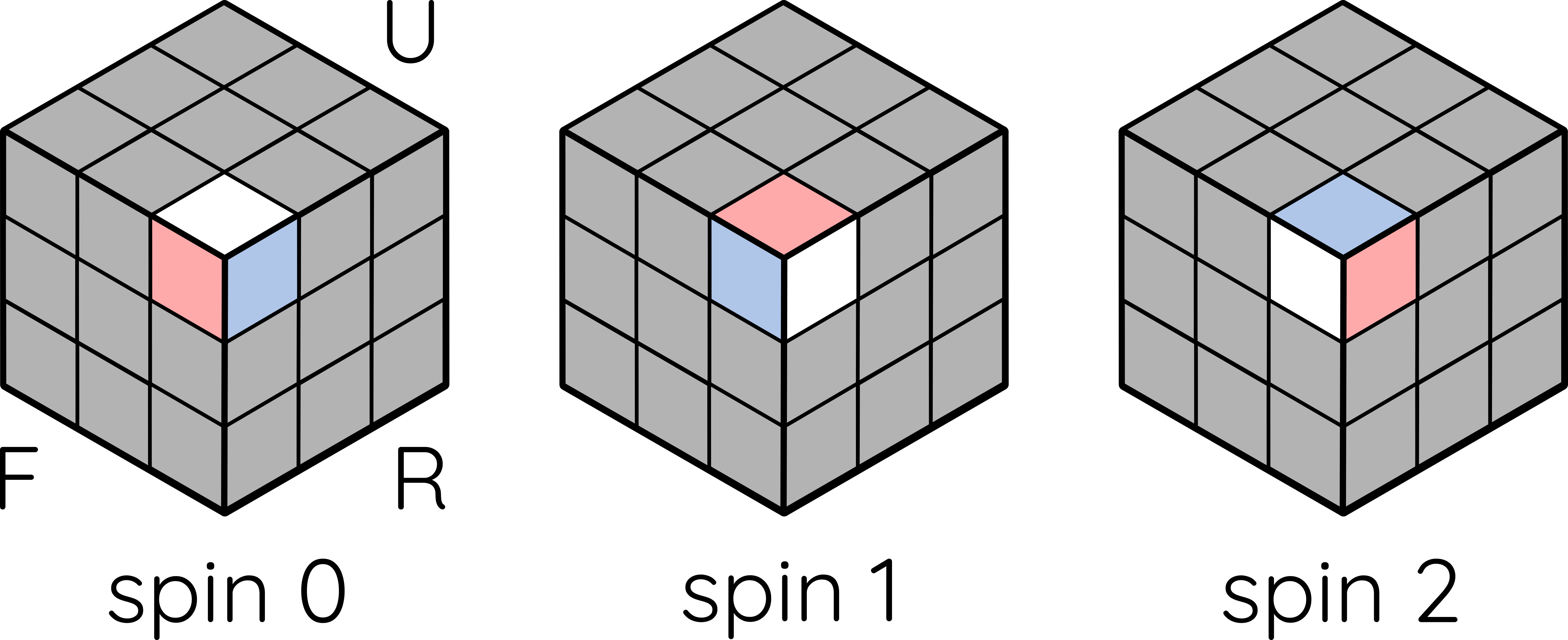
A series of definitions need to be made. In an homage to physics, the orientation properties of corners and edges are named spin and parity respectively. Instead of half spins in physics, a corner has 3 spin states: when its white/yellow face is facing top/bottom, spin is 0. Twisting it clockwise once gives spin 1; twice, spin 2.

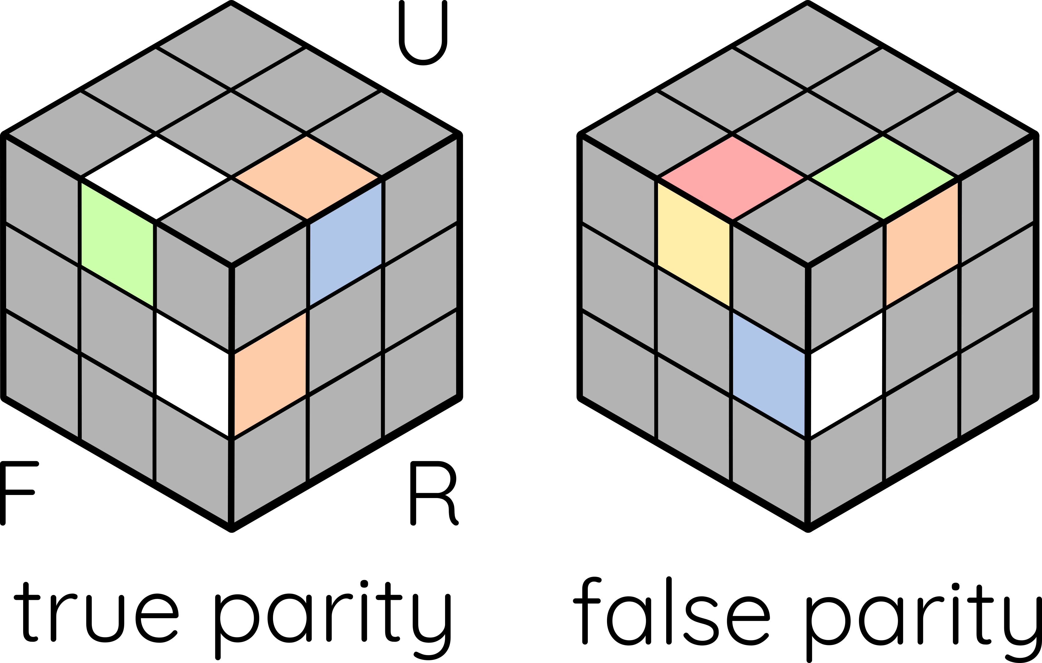
Parity is a little bit more complicated. Each edge has two faces, and we have to designate one as the “principal face”: if an edge has a white/yellow face, then that face is principal; if not, then the red/orange face will be principal. When an edge is in the top/bottom layer, parity is true when the principal face is facing top/bottom, false if not; if an edge is in the equatorial layer, then parity is true when the principal face is facing the front/back, false if facing the sides.

You will later see how these definitions of spin and parity help us identify cases and systematically solve the cube. But its first application is turning a single face: 4 edges and 4 corners will cycle, and 4 parities and spins will change. Note that while we could have coded it such that orientations will always follow the cubie instead of the location, linking it to the location is, again, efficient for case identification.

CFOP

I have to say straight out of the gate, that all intuitive steps in solving the cube were done algorithmically. I did not have time to write a search algorithm, and therefore all intuitive steps were not optimized. I am very sorry.

The white cross was inserted corner by corner, and on average it takes about 11 moves, significantly more than the 6 moves that if we were inserting intuitively. The error was taken into account when analyzing the data.

However, it is much easier to execute algorithmic steps using code. Every step is split into 3 substeps: obtainment (of information), identification (of case), and execution (of algorithm). As I am still a beginner at Java, the code is particularly messy in the beginning.

There are only 4 things that we needed to obtain to complete a single F2L pair: the positions & orientations of said corner & edge pair. While there are many F2L algorithms out there on the internet, we realized that they only work when said pair is either in position or in the top layer. This adds a layer of complexity, as we needed to identify whether “extraction” is needed to move all the needed pieces to the top layer. But after extracting the material, there are simply 42 cases in the decision tree, and an algorithm is fed into the code for it to choose.

OLL is a little bit more curious. In cuber terms, this step correctly orients all of the top layer; similarly in code, this step makes the entire cube spin 0 and true parity. The information we needed was the 8 orientations of the top layer. However, this time, the decision tree for case identification is a lot more complicated, as the computer cannot intuitively identify P-, W-, awkward cases, et cetera. Much time was spent on planning, as correctly identifying every feature for similar cases was difficult for the human eye.

After the fiasco that is the 57 cases of OLL, PLL is relatively easy. Only the 8 positions are considered, and to a certain extent, this is similar to identifying F2L cases. There is nothing too special about this step.

Roux

As I have said earlier, intuitive steps are not optimized. Due to constraints in time, F2B is completed using white cross and F2L algorithms.

The third step of Roux is to orient and permute corners of the top layer. A similar approach as OLL & PLL is taken, but this time using CMLL algorithms.

L6E is slightly different. It is considered a “semi-intuitive” step, so while EOLR can be partly executed using our parity and position information, actually inserting LR and finishing the middle slice permutation requires detailing of all four cases.

Regrips

3 out of the 4 factors that we keep track of are simple counters. However, regrips are a little bit difficult to quantify. To solve the problem, we simply simulate all the possible hand positions given a set of moves, and when there is an inevitable change in hand position, then a regrip must exist. Since with some moves, there is a multitude of hand positions possible; with that, in another nod to physics, we say that you are in a superposition, a combination of possible hand positions represented in arrays, until we get more specifics, and it collapses back to a single possible hand position.

Scrambles

While there are existing official computer program scramblers, none of them spit the scrambles out nicely in a single text file. So, I wrote a small file that generates a random length, random (with some constraints) move sequence. With that, the program can read the scrambles line by line and use the solvers that we spent so much time on.

Putting It All Together

Once the 10 weeks of painful coding was over, data taking was relatively simple, as predicted initially. We tested multiple numbers of scrambles & solves, and found out pretty quickly that our code was relatively efficient. We settled on 1 million solves as our data set, as data taking at that point takes less than 3 minutes. Also, we did not want to exceed to Microsoft Excel row limit, because otherwise we would have to write our own analysis software, which meant more coding, which implies more work and… 1 million solves was ideal.

I was pretty surprised that the graphs turned out to be pretty nice, and the normal curves looked pretty continuous for a discrete data set.

Final Thoughts

In the forseeable future (summer), I would like to revisit the No-Regrips factor, maybe add more methods, probably add a UI for completeness’ sake, and of course, make a third update after all of that is done.

Overall, coding this project was pretty fun. I would like the extend a token of thanks to:

• Callum Lehingrat, without whom this project will not be complete;
• Gwen Kornak, who provided much needed help with Java; and
• all of Science One, who supported us throughout.

Thank you very much for reading all of this. Stay tuned for more updates.